Car Detection With Yolov2 Try Again Âⷠ3040 Points Earned You Must Earn 3240 Points to Pass

Guide to Car Detection using YOLO

In-depth concept of the YOLO algorithm — bounding boxes, not-max suppression and IOU.

Existent-time object detection using YOLOv3

1. Problem Statement

You are working on a self-driving car. As a critical component of this project, you lot'd similar to first build a auto detection system. To collect data, you've mounted a camera to the hood of the car, which takes pictures of the road ahead every few seconds while you drive effectually.

Pictures taken from a car-mounted camera while driving effectually Silicon Valley.
Thanks to drive.ai for providing this dataset.

You lot've gathered all these images into a folder and have labelled them by drawing bounding boxes around every car yous plant. Here's an example of what your bounding boxes look like:

Figure i: Definition of a bounding box

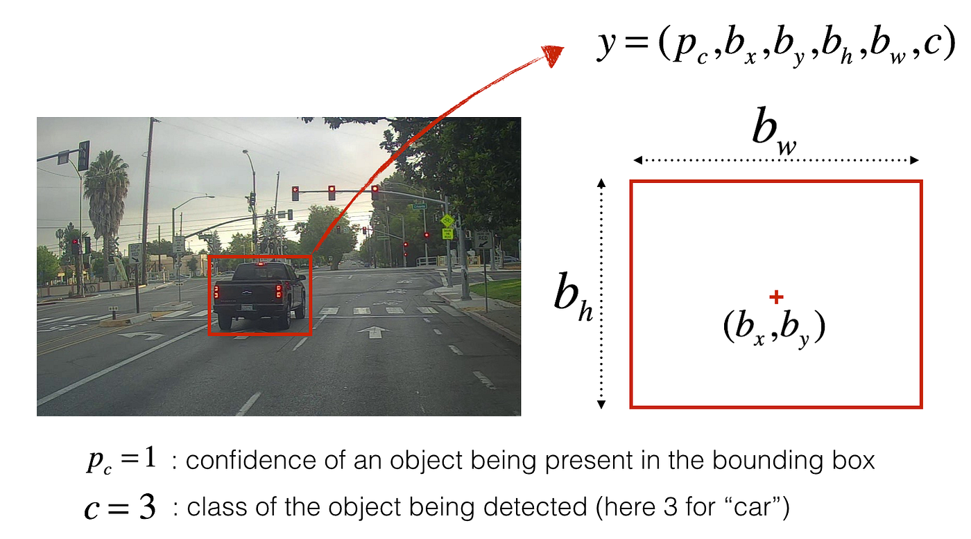
If you have 80 classes that you want the object detector to recognize, yous can stand for the class label c either equally an integer from ane to 80, or as an fourscore-dimensional vector (with 80 numbers) — one component of which is one and the rest of which are 0. In this article, I volition be using both representations, depending on which is more convenient for a particular step.

ii. YOLO

"You lot Only Look Once" (YOLO) is a popular algorithm because it achieves high accurateness whilst besides being able to run in real-time. This algorithm "only looks once" at the image in the sense that it requires only one forward propagation pass through the network to brand predictions. Subsequently non-max suppression, it then outputs recognized objects together with the bounding boxes.

ii.1 Model details

Inputs and outputs

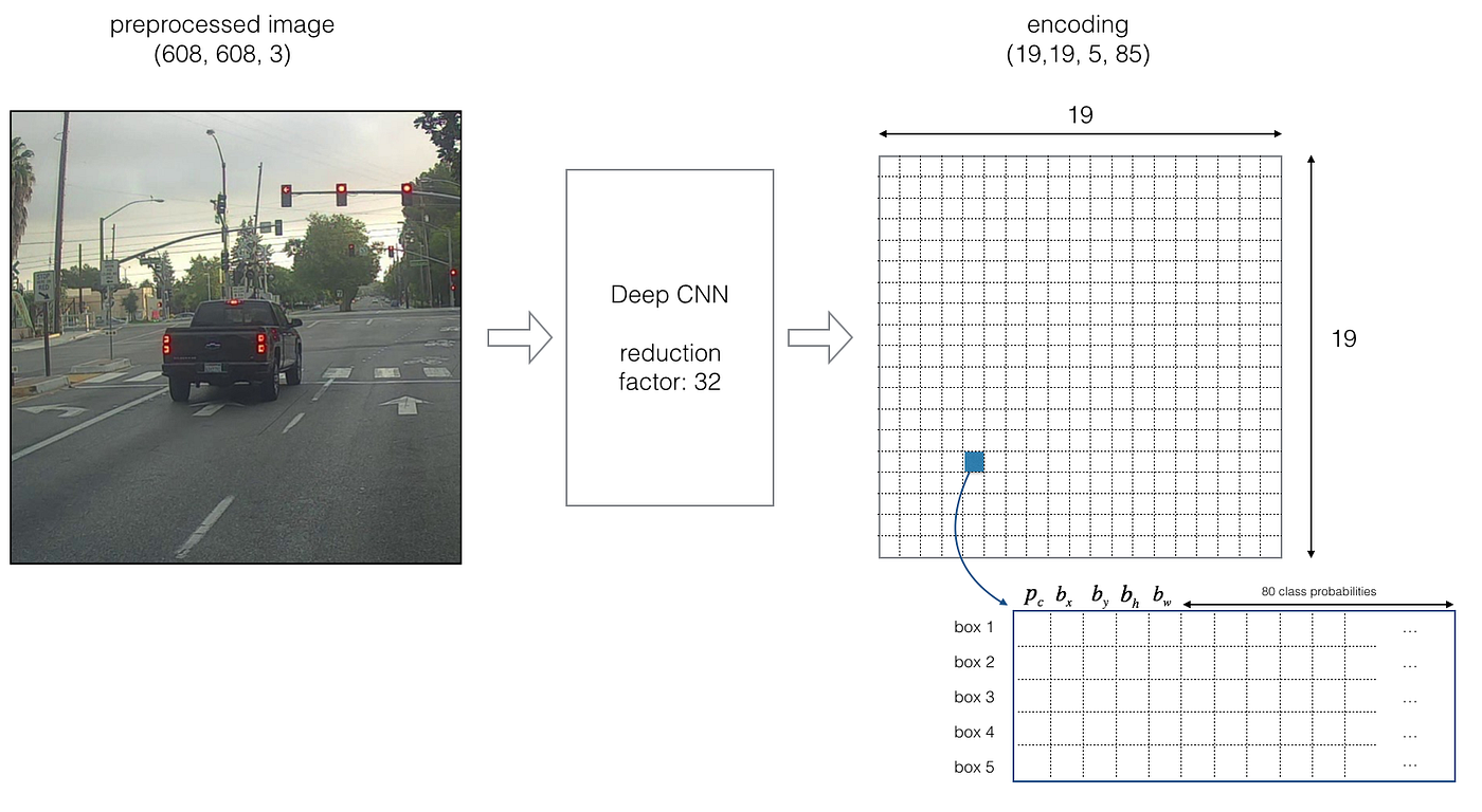
• The input is a batch of images, and each image has the shape (m, 608, 608, iii).
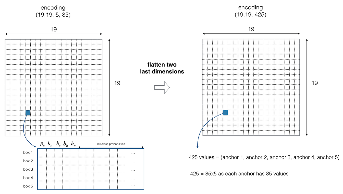
• The output is a list of bounding boxes forth with the recognized classes. Each bounding box is represented by half dozen numbers — pc, bx, by, bh, bw, c — as explained above. If you expand c into an 80-dimensional vector, each bounding box is so represented past 85 numbers.

Anchor Boxes

• Ballast boxes are chosen by exploring the grooming data to cull reasonable height/width ratios that represent the different classes.
• The dimension for anchor boxes is the second to last dimension in the encoding: m, nH, nW, anchors, classes.
• The YOLO architecture is: IMAGE (thou, 608, 608, three) -> DEEP CNN -> ENCODING (m, 19, nineteen, five, 85).

Encoding

Allow'due south look in greater item at what this encoding represents.

Effigy two: Encoding compages for YOLO

If the center/midpoint of an object falls into a grid cell, that grid cell is responsible for detecting that object.

Since we are using 5 ballast boxes, each of the 19 x 19 cells thus encodes information well-nigh five boxes. Ballast boxes are defined only by their width and height.

For simplicity, we will flatten the last two last dimensions of the shape (19, xix, 5, 85) encoding. And so the output of the Deep CNN is (19, xix, 425).

Figure 3: Flattening the last two last dimensions

Form score

Now, for each box (of each cell), we will compute the following element-wise product and excerpt a probability that the box contains a sure class.

The form score is score_cᵢ = p_c * cᵢ — the probability that at that place is an object p_c times the probability that the object is a certain form cᵢ.

Effigy 4: Observe the class detected by each box

In Figure four, permit's say for box ane (cell ane), the probability that an object exists is p₁ = 0.lx. So at that place's a 60% risk that an object exists in box ane (jail cell 1).

The probability that the object is the class category 3 (a car) is c₃ = 0.73.

The score for box 1 and for category three is score_c₁,₃ = 0.sixty * 0.73 = 0.44.

Let's say we summate the score for all 80 classes in box 1 and notice that the score for the auto class (class 3) is the maximum. Then nosotros'll assign the score 0.44 and course iii to this box one.

Visualizing classes

Here's one way to visualize what YOLO is predicting on an image:

• For each of the 19 x 19 filigree cells, observe the maximum of the probability scores, that is, taking a max across the 80 classes, one maximum for each of the 5 anchor boxes).
• Colour that filigree cell according to what object that grid prison cell considers the most likely.

Doing this results in this film:

Figure 5: Each one of the 19 ten 19 grid cells is coloured according to which form has the largest predicted probability in that cell.

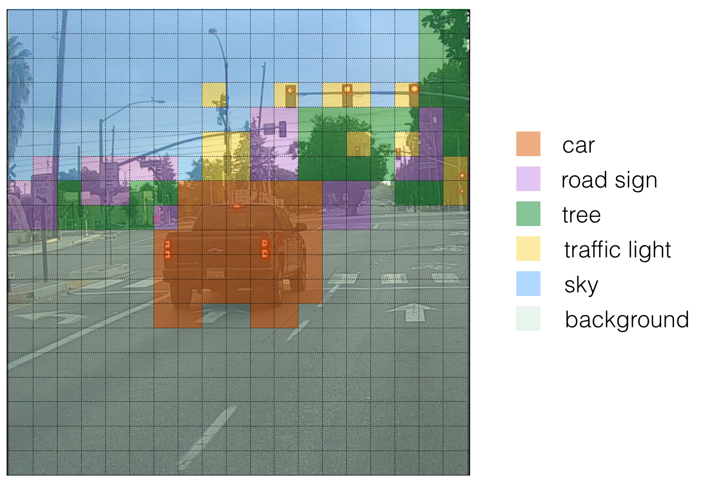
Note that this visualization isn't a core function of the YOLO algorithm itself for making predictions; it'southward just a squeamish way of visualizing an intermediate event of the algorithm.

Visualizing bounding boxes

Another way to visualize YOLO's output is to plot the bounding boxes that it outputs. Doing that results in a visualization like this:

Effigy 6: Each cell gives you 5 boxes. In total, the model predicts 19x19x5 = 1805 boxes but by looking in one case at the image (one forwards pass through the network)! Different colours announce different classes.

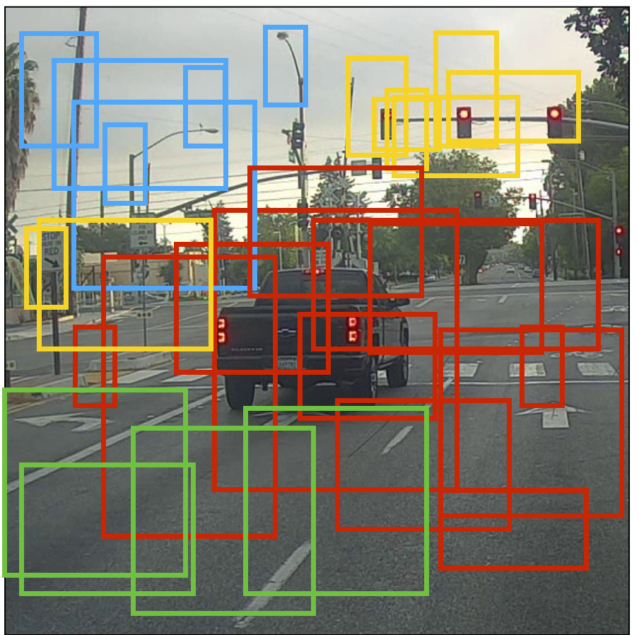
Non-Max suppression

In the figure above, nosotros plotted but boxes for which the model had assigned a high probability, merely this is still too many boxes. We'd like to reduce the algorithm'south output to a much smaller number of detected objects.

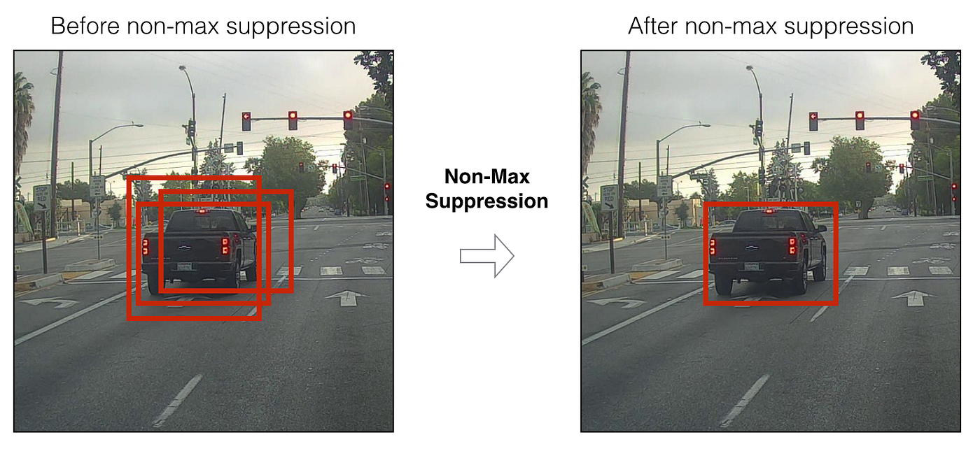
To do so, nosotros'll use not-max suppression. Specifically, we'll carry out these steps:

• Get rid of boxes with a low score. Meaning, the box is not very confident about detecting a grade; either due to the depression probability of any object, or depression probability of this particular class.
• Select simply i box when several boxes overlap with each other and detect the same object.

2.ii Filtering with a threshold on class scores

We are going to first apply a filter by thresholding. We would like to become rid of whatsoever box for which the class "score" is less than a chosen threshold.

The model gives united states of america a full of 19 x 19 x 5 10 85 numbers, with each box described by 85 numbers. It is convenient to rearrange the (19, 19, 5, 85), or (19, xix, 425) dimensional tensor into the following variables:

• box_confidence: tensor of shape (nineteen×19, v, 1)(19×19, 5, 1) containing p_c — conviction probability that in that location's some object — for each of the five boxes predicted in each of the 19x19 cells.
• boxes: tensor of shape (nineteen×xix, five, iv) containing the midpoint and dimensions (bx, by , bh, bw) for each of the v boxes in each jail cell.
• box_class_probs: tensor of shape (19×nineteen, 5, 80) containing the "class probabilities" (c₁, c₂,…,c₈₀) for each of the 80 classes for each of the five boxes per prison cell.

Implementing yolo_filter_boxes()

1. Compute box scores by doing the element-wise product(p * c) every bit described in Figure 4.
2. For each box, discover the index of the grade with the maximum box score, and the corresponding box score.
3. Create a mask past using a threshold. As a heads-upward: ([0.9, 0.3, 0.four, 0.5, 0.i] < 0.4) returns: [Fake, Truthful, False, Imitation, True]. The mask should be True for the boxes you want to continue.
4. Use TensorFlow to apply the mask to box_class_scores, boxes and box_classes to filter out the boxes nosotros don't want. You should be left with just the subset of boxes you lot desire to keep.

Useful references

• Keras argmax
• Keras max
• boolean mask

2.3 Non-max suppression

Even after filtering by thresholding over the class scores, we might notwithstanding stop up with a lot of overlapping boxes. A second filter for selecting the right boxes is called non-maximum suppression (NMS).

Figure 7: In this instance, the model has predicted three cars, but information technology'south actually three predictions of the aforementioned motorcar. Running non-max suppression (NMS) will select only the near accurate (highest probability) of the 3 boxes.

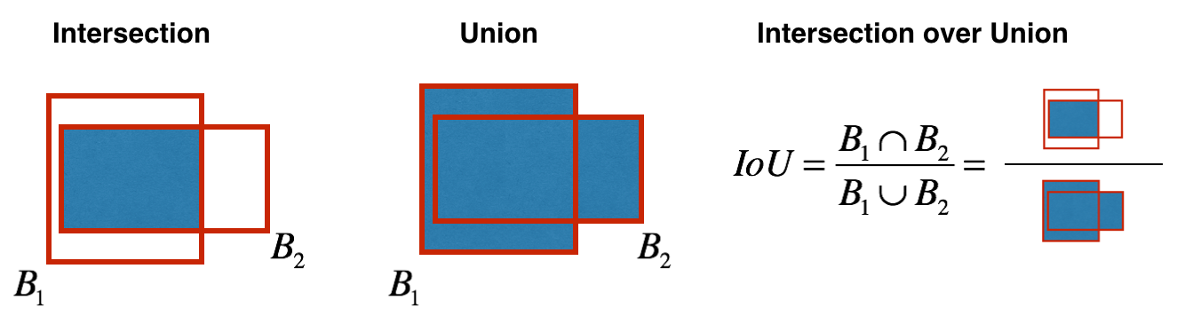
Non-max suppression uses the very crucial function called Intersection over Union, or IoU.

Effigy 8: Definition of Intersection over Matrimony.

Implementing iou()

In this code, I'll be using the convention that (0, 0) is the superlative-left corner of an image; (1, 0) is the upper-correct corner; (ane, one) is the lower-right corner. In other words, the (0, 0) origin starts at the top left corner of the prototype. As x increases, we movement to the right. As y increases, we motility downwards.

I'll define a box using its two corners: upper left (x₁, y₁) and lower right (x₂, y₂) instead of using the midpoint, pinnacle and width. This makes it a bit easier to calculate the intersection.

To calculate the expanse of a rectangle, multiply its top (y₂ − y₁) by its width (x₂ − x₁). Since (10₁, y₁) is the top left and (ten₂, y₂) is the lesser right, these differences should be non-negative.

Feel free to draw some examples on paper to clarify this conceptually. To find the intersection of the two boxes (xi₁, yi₁, xi₂, yi₂):

• The top left corner of the intersection (xi₁, yi₁) is plant by comparing the meridian left corners (x₁, y₁) of the two boxes, and so finding a vertex that has an x-coordinate that is closer to the right, and y-coordinate that is closer to the lesser.
• The bottom correct corner of the intersection ( xi₂, yi₂) is plant past comparison the bottom right corners (x₂, y₂) of the 2 boxes, then finding a vertex whose x-coordinate is closer to the left, and the y-coordinate that is closer to the top.
• The two boxes may accept no intersection. Nosotros tin find this if the intersection coordinates nosotros calculated end up being the top correct and/or lesser left corners of an intersection box. Some other way to think of this is if you lot calculated the height (y₂ − y₁) or width (x₂ − 10₁) and observe that at least ane of these lengths is negative, so at that place is no intersection (intersection area is zero).
• The ii boxes may intersect at the edges or vertices, in which example the intersection area is yet zippo. This happens when either the superlative or width (or both) of the calculated intersection is zero.

YOLO non-max suppression

We are now ready to implement non-max suppression. The key steps are:

1. Select the box that has the highest score.
2. Compute the overlap of this box with all other boxes, and remove boxes that overlap significantly (iou >= iou_threshold).
3. Go back to step 1 and iterate until there are no more than boxes with a lower score than the currently selected box.

This volition remove all boxes that have a large overlap with the selected boxes. Simply the "best" boxes remain.

Implementing yolo_non_max_suppression()

Reference documentation

• tf.image.non_max_suppression()

ii.4 Wrapping up the filtering

It's time to implement a function taking the output of the deep CNN (the 19 x 19 x 5 x 85 dimensional encoding) and filtering through all the boxes using the functions we've only implemented.

Implementing yolo_eval()

This function takes the output of the YOLO encoding and filters the boxes using score threshold and NMS.

In that location's one implementations detail you need to know. At that place are a few ways of representing boxes, such equally via their corners or via their midpoint and elevation/width. YOLO converts between a few such formats at different times, using the post-obit functions:

          boxes = yolo_boxes_to_corners(box_xy, box_wh)        

which converts the YOLO box coordinates (x, y, w, h) to box corners' coordinates (10₁, y₁, ten₂, y₂) to fit the input of yolo_filter_boxes .

          boxes = scale_boxes(boxes, image_shape)        

YOLO's network was trained to run on 608 x 608 images. If you are testing this data on a different size image — for instance, a car detection dataset with 720 x 1280 images — this step rescales the boxes so that they tin exist plotted on top of the original 720 10 1280 image.

2.5 Summary for YOLO

• Input image (608, 608, 3)
• The input image goes through a CNN, resulting in a (xix, xix, v, 85) dimensional output.
• Afterward flattening the terminal two dimensions, the output is a volume of shape (19, 19, 425). Each cell in a 19 x 19 grid over the input epitome gives 425 numbers: 425 = 5 x 85 because each cell contains predictions for v boxes, corresponding to 5 anchor boxes; 85 = 5 + eighty where 5 is because (pc, bx, past, bh, bw) has 5 numbers, and lxxx is the number of classes we'd like to find.
• We and then select but a few boxes based on score-thresholding — discarding boxes that have detected a class with a score less than the threshold, and non-max suppression — calculating the Intersection over Union (IOU) and avoiding selecting overlapping boxes.
• This gives you lot YOLO'south last output.

iii. Testing YOLO pre-trained model on images

In this role, we are going to apply a pre-trained model and exam it on the car detection dataset. Nosotros'll need a session to execute the computation graph and evaluate the tensors:

          sess = K.get_session()        

3.1 Defining classes, anchors and prototype shape

Recall that we were trying to observe 80 classes, and are using 5 anchor boxes. Nosotros will read the names and anchors of the fourscore classes and 5 boxes that are stored in two files — coco_classes.txt and yolo_anchors.txt (more info in Github repo). The automobile detection dataset has 720 10 1280 images, which are pre-candy into 608 10 608 images.

iii.2 Loading a pre-trained model

Preparation a YOLO model takes a very long fourth dimension and requires a adequately large dataset of labelled bounding boxes for a large range of target classes. And so we are instead going to load an existing pre-trained Keras YOLO model. (more info in Github repo). These weights come from the official YOLO website and were converted using a office written by Allan Zelener. References are at the stop of this article. Technically, these are the parameters from the YOLOv2 model, but we will simply refer to information technology equally YOLO in this commodity.

          yolo_model = load_model("model_data/yolo.h5")        

This loads the weights of a trained YOLO model. Yous can take a look at the summary of the layers the model contains in the notebook in the Github repo.

Reminder: this model converts a preprocessed batch of input images (shape: (1000, 608, 608, 3)) into a tensor of shape (one thousand, 19, 19, five, 85) as explained in Figure 2.

three.3 Convert output of the model to usable bounding box tensors

The output of yolo_model is a (m, 19, 19, 5, 85) tensor that needs to pass through not-trivial processing and conversion. The post-obit code does that for united states:

          yolo_outputs = yolo_head(yolo_model.output, anchors, len(class_names))        

If y'all are curious most how yolo_head is implemented, you can detect the function definition in the file 'keras_yolo.py' in the Github repo.

Subsequently adding yolo_outputs to our graph. This set up of four tensors is ready to be used as input by the yolo_eval role.

3.four Filtering boxes

yolo_outputs gave us all the predicted boxes of yolo_model in the correct format. We're at present ready to perform filtering and selecting only the all-time boxes by calling yolo_eval, which we had previously implemented, to practise this.

          scores, boxes, classes = yolo_eval(yolo_outputs, image_shape)        

iii.5 Run the graph on an paradigm

Let the fun brainstorm. We accept created a graph that can be summarized as follows:

1. yolo_model.input is given to yolo_model. The model is used to compute the output yolo_model.output.
2. yolo_model.output is processed by yolo_head. It gives you yolo_outputs.
3. yolo_outputs goes through a filtering office, yolo_eval. Information technology outputs your predictions: scores, boxes, classes.

Implementing predict()

predict() runs the graph to exam YOLO on an prototype. Y'all will need to run a TensorFlow session, to have it compute scores, boxes, classes.

The code below also uses the post-obit role:

          image, image_data = preprocess_image("images/"            +            image_file, model_image_size = (608, 608))        

which outputs:

• image: a python (PIL) representation of your image used for drawing boxes. You won't need to use it.
• image_data: a numpy-array representing the image. This will be the input to the CNN.

Testing the function on a test prototype:

          out_scores, out_boxes, out_classes = predict(sess, "test.jpg")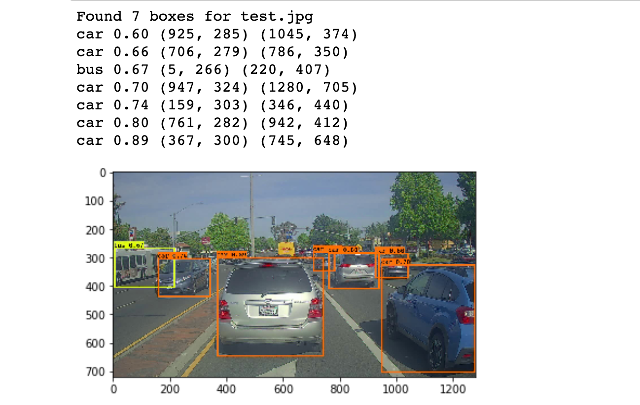        

Example output on test.jpg

The model we've simply run is actually able to discover eighty different classes listed in coco_classes.txt. Feel free to try with on with your own images by downloading the files in the Github repo.

If nosotros were to run the session in a for loop over all the images. Here'southward what we would become:

4. Conclusion

• YOLO is a land-of-the-art object detection model that is fast and accurate.
• It runs an input image through a CNN which outputs a 19 x 19 10 5 x 85 dimensional volume.
• The encoding tin can be seen as a filigree where each of the 19 ten 19 cells contains information about 5 boxes.
• Filter through all the boxes using non-max suppression. Specifically, use score thresholding on the probability of detecting a class to go along merely accurate (loftier probability) boxes, and Intersection over Union (IoU) thresholding to eliminate overlapping boxes.
• Because training a YOLO model from randomly initialized weights is non-niggling and requires a big dataset equally well as a lot of computation, we used previously trained model parameters in this exercise. If yous wish, y'all tin can also effort fine-tuning the YOLO model with your own dataset, though this would be a adequately non-piddling practice.

Citations & References

Special thanks to deeplearning.ai.

All figures by courtesy of deeplearning.ai.

The ideas presented in this article came primarily from the two YOLO papers. The implementation here also took significant inspiration and used many components from Allan Zelener's GitHub repository. The pre-trained weights used in this exercise came from the official YOLO website.

• Joseph Redmon, Santosh Divvala, Ross Girshick, Ali Farhadi — You lot Just Look In one case: Unified, Real-Time Object Detection (2015)
• Joseph Redmon, Ali Farhadi — YOLO9000: Meliorate, Faster, Stronger (2016)
• Allan Zelener — YAD2K: Yet Some other Darknet 2 Keras
• The official YOLO website (https://pjreddie.com/darknet/yolo/)

Car detection dataset: The Bulldoze.ai Sample Dataset (provided by drive.ai) is licensed under a Artistic Eatables Attribution 4.0 International License.

Github repo: https://github.com/TheClub4/motorcar-detection-yolov2

morganthedidismind84.blogspot.com

Source: https://towardsdatascience.com/guide-to-car-detection-using-yolo-48caac8e4ded

Share this post